Flory-Huggins Theory
for Inhomogeous Systems
The Flory-Huggins mean-field theory is one of the most popular theories in polymer physics and has been described in great detail in many polymer physics books. It was developed by Paul Flory1 and Maurice Huggins2 independently in the early 1940s as an extension of the lattice fluid theory which was originally developed to describe the miscibility and phase separation behavior of low-molecular-weight liquids.
Despite its tremendous success, the classical Flory-Huggins theory has also some limitations. For example, the equations derived by Flory and Huggins are only applicable to homogenous polymer solutions and melts. In other words, they cannot be applied to systems with a macroscopic concentration gradient as is the case for polymers near liquid-liquid and liquid-solid interfaces. This problem was first solved by Ryong-Joon Roe in the early 1970s.4
Two-dimensional Lattice
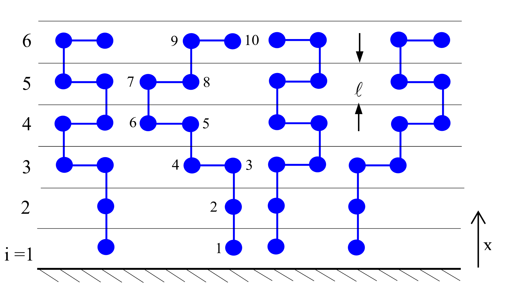
Two-dimensional Lattice
Like Flory, Roe assumed a rigid lattice frame
which he devided into M layers of L lattice sites parallel to the (solid
or liquid)
interface. The total number of lattice sites, N0 = ML, was assumed to be equal to
the number of solvent molecules, Ns, and
polymer repeat units, Npr:
![]()
where Np is the number of polymer molecules, each consisting of r repeat units. Furthermore, the field in which the r-mers and solvent molecules reside was assumed to be self-consistent.
The number of ways of placing the Ns solvent molecules on the ML latice sites is given by
![]()
and the number of ways of arranging Np r-mers on the remaining ML- Ns is given by
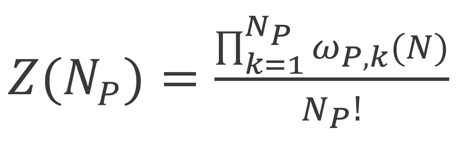
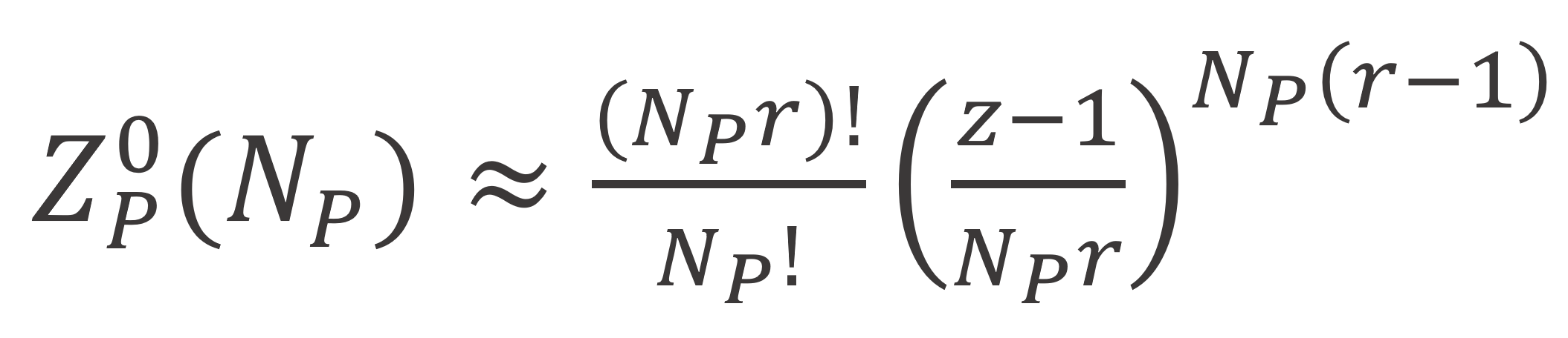
Here ωp,k is the number of ways of placing a r-mer molecule after Ns solvent molecules and (k-1) r-mers have already been placed on the lattice. Roe chose as a reference state the melt-state for which Flory derived following expression:3
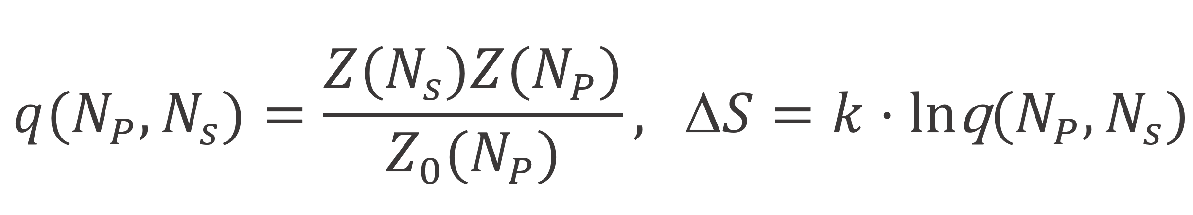
With these three expressions, the total number of arrangements and the corrsponding entropy can be calculated as follows:
Thus to calculate the entropy of mixing, we first need to find expressions for ωP,k which can be derived with the Bragg-Williams approximation of random mixing.10 Roe found4,6

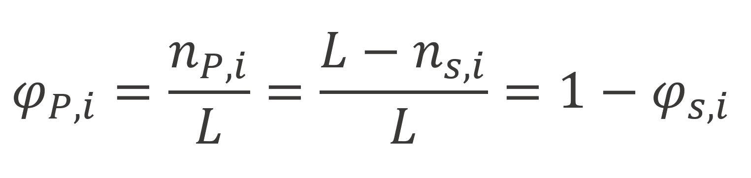
here nP,i is the total number of polymer segments in the i-th layer, λo, λ1 are lattice parameters and φP,i = 1 - φs,i is the segment volume fraction in the i-th layer,
Combining the expressions above, we obtain:
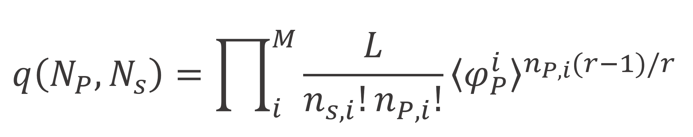
where ⟨φP,i⟩ is defined by
![]()
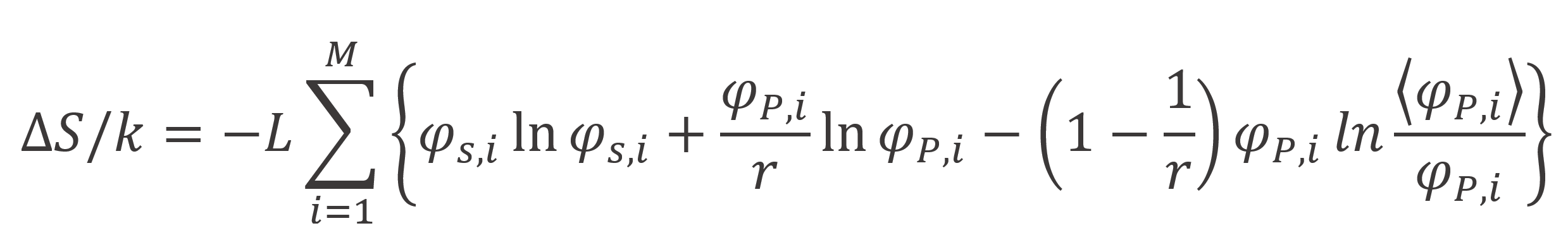
Taking the logarithm and using the Stirling formula we find following expression for the entropy of mixing in the vicinity of an interface:
Helfland5 and Scheutjens and Fleer6,7 pointed out that Roe's derivation disregards the inversion symmetry, which requires that a conformation starting with s = 1 at z is identical with the inverted one, where s = r at z. This symmetry is automatically obeyed when using Fleer's and Scheutjens' composition law:6,7
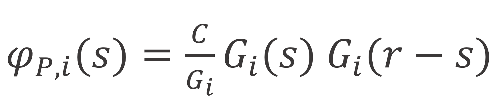
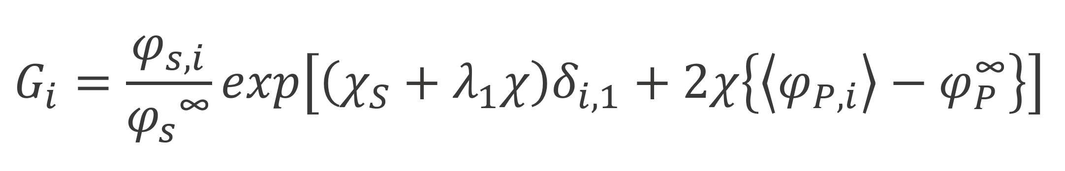
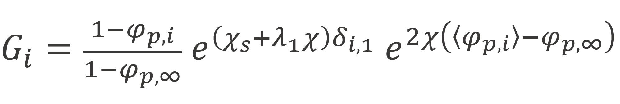
where C is normalization constant, which can be determined from the boundary condition of the end points: φP∞(s) = φP∞ / N, and Gi is a correction for double counting, called segment weighting factor which has the value
The total amount of polymer segments in the i-th layer is given by summation of φP(s) over all segments s = 1, 2,...,r -1, r:
![]()
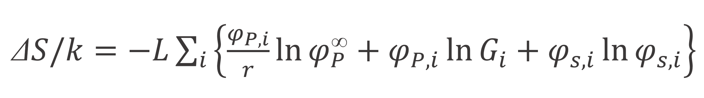
Using the inversion symmetry, Scheutjens and Fleer found folowing expression for the entropy of mixing6,7
The inhomogenous distributuion of segments in the vicinity of the interface originates from the interaction of r-mers with the (solid) surface. The corresponding excess energy is given by -χS L φ1, where χS = (u - us) / kT is the dimensionless adsorption energy parameter, also called Silberberg parameter.
The mixing of polymer segments with solvent molecules causes a change in energy. This energy can be calculated with the Flory-Huggins mean-field theory using the Braggs-Williams approximation,10

Then the total energy due to absorption and mixing reads,6,7
![]()
To calculate the polymer volume profile and the respective entropy and energy, we first need to calculate all end segment probabilities, Gi(s). This can be done with DiMarzio's transition matrix method by chosing as a starting vector G(1) = {G1, ...,Gi,...GM} and by replacing the matrix elements λ0 and λ1 by λ0Gi and λ1Gi. The Gi values required for this method can be calculated from
The N segement probabilities Gi(s) can then be determined recursively from
![]()
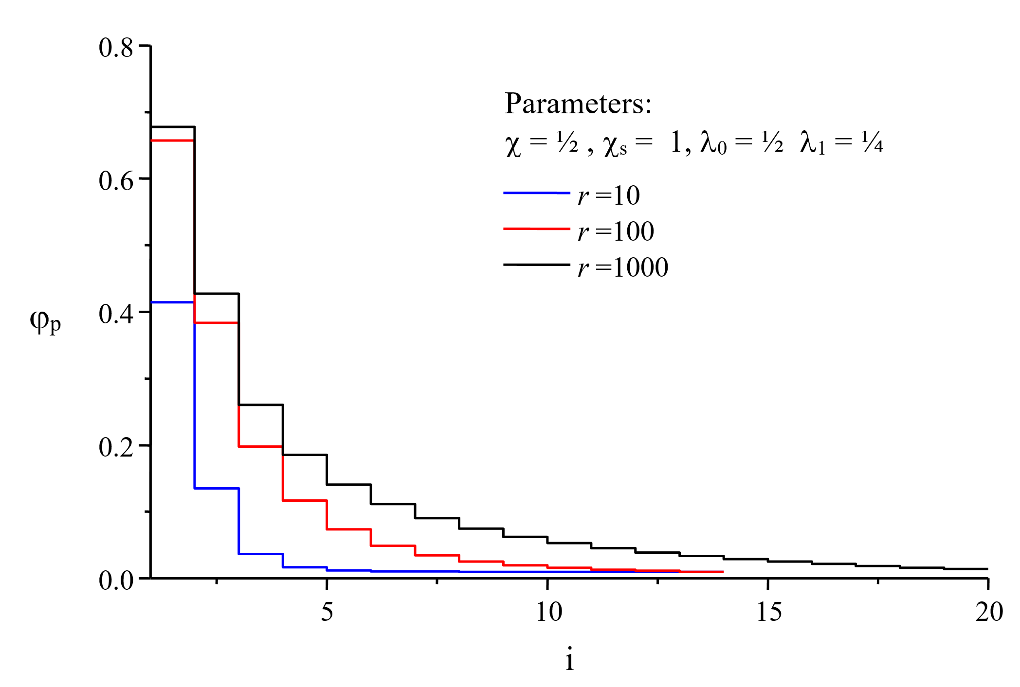
However, this is a rather difficult task, since the polymer volume fractions are unknown. In general, this problem can be only solved by a multidimensional iteration procedure.8 The concentration profile obtained by this method is shown in the figure below for three different chain lengths r.
Alternatively, a ground state approximation can be employed that allows for a direct estimate of the polymer concentrarion profile, as will be shown elsewhere. However, this method is only applicable to the polymer concentration profile near the interface.9
References & Further Readings
P. J. Flory, J. Chem. Phys. 9, 660 (1941); 10, 51 (1942)
M. L. Huggins, J. Phys. Chem. 46, 151 (1942); J. Am. Chem. Soc. 64, 1712 (1942)
Paul L. Flory, Principles of Polymer Chemistry, Ithaca, New york, 1953
R. J. Roe, J. Chem. Phys. 60, 4192 (1974)
E. Helfland, J. Chem. Phys. 63, 2192 (1974), Macromolecules 9, 307 (1976)
J.M. Scheutjens, G.J. Fleer, J. Phys. Chem. 83, 1620 (1979) & 84, 178 (1980)
G.J. Fleer, M.A. Cohen Stuart, J.M.H.M. Scheutjens, T. Cosgrove, B. Vincent; Polymers at Intefaces; Chapman & Hill, Cambridge (GB) 1993
V. Hanagandi, H. Ploehn, M. Nikolaou, Chem. Engin. Sci., 51(7), 1071-1078 (1996)
G.J. Fleer, and F.A.M. Leermakers, Macromol. Symp. 126, 65 (1997)
The Bragg—Williams approximation, also called the mean-field approximation, reduces a many-body problem into an effective one-body problem. In this theory all interactions with neighboring molecules are replaced with an average or effective interaction, sometimes called a molecular mean-field. This approximation is especially useful for complex multi-body problems such as phase transition phenomena.